Previously we have tried logistic regression without regularization and with the simple training data set. But as we all know, things in real life aren’t as simple as we would want to. There are many types of data available that need to be classified. A number of features can grow up hundreds and thousands while a number of instances may be limited. Also in, many times, we might need to classify into more than two classes.
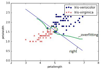
The first problem that might arise due to many features is over-fitting. This is when learned hypothesis hΘ (x) fit training data too well (cost J(Θ) ≈ 0), but it fails when classifying new data samples. In other words, the model tries to distinct each training example correctly by drawing very complicated decision boundaries between training data points.

As you can see in the image above, over-fitting would be green decision boundary. So how to deal with the over-fitting problem? There might be several approaches:
- Reducing the number of features;
- Selecting different classification models;
- Use regularization.
We leave first two out of the question because selecting an optimal number of features is a different topic of optimization. Also, we are sticking with logistic regression model for now, so changing classifier is also out of the question. We choose third option, which is the more general and proper way of addressing the problem.
Regularized cost function and gradient descent
In order to regularize cost function we need to add penalization to it. Mathematically speaking, we need to add norm of parameter vector multiplied with regularization parameter λ. By selecting regularization parameter, we can fine-tune the fitting.
This is cost function with regularization:

And similarly gradient function:

We can see that parameter Θ0 should now be regularized.
The other procedure remains same – we need to minimize JΘuntil we converge.
Python code of cost function:
def cost(theta, X, y, lmd):
    '''  regularized logistic regression cost    '''
    sxt = sigmoid(np.dot(X, theta));
    mcost = (-y)*np.log(sxt) - (1-y)*np.log(1-sxt) + lmd/2 * np.dot(theta.T,theta);
    return mcost.mean()
Feature normalization
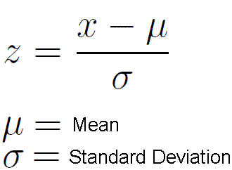
A good practice is to normalize training data in order to bring scales to a similar level. This makes optimization tasks easier and less intense. For manual operations, you could use mean normalization (sometimes called Z score):

If you don’t want to waste time coding, then use scale function from scikit-learn library. As you progress further, you will find that all tools and functions required for most of machine-learning tasks can be found in this library.
from sklearn import svm, preprocessing
#...
XN = preprocessing.scale(X);
For optimization of Θ, we are going to use a function called fmin_bfgs, which takes cost function, initial thetas, and produces thetas of minimized function. This is same as previously; the only new thing is lambda parameter which should be included in the parameter list.
#create initial theta values
theta = 0.1* np.random.randn(n);
#initial lambda
lmd = 0.005;
#use fmin_bfgs optimisation function find thetas
theta = opt.fmin_bfgs(cost, theta, args=(XX, Y, lmd));
Evaluating logistic regression classifier with regularization
This time we will use a more complex data set downloaded from kaggle.com. The data set consists of 569 instances having 30 features. Features are calculated from actual cell nucleus digitized images taken from breast mass using fine needle aspirate (FNA).
a) radius (mean of distances from the center to points on the perimeter) b) texture (standard deviation of gray-scale values) c) perimeter d) area e) smoothness (local variation in radius lengths) f) compactness (perimeter^2 / area – 1.0) g) concavity (severity of concave portions of the contour) h) concave points (number of concave portions of the contour) i) symmetry j) fractal dimension (“coastline approximation” – 1)
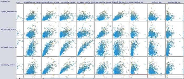
It is hard to plot data sets in one plot; this might be done by plotting plot matrix where each pair of features might be represented. Also, this could be done with 3D graphs. This is a fragment of plot matrix:

Each patient has a marker, either it is malignant or benign. In order to teach classifier and test it, we split the database into two sets – training set and test set. By applying test set to built model, we can validate if the model is good.
A running model with a test set, we get Accuracy: 98.1%.
Algorithm and data sets for your own try is here: logistic_regression_reg

