
Some may say that linear regression is a more statistical problem. And this is true at some level. But when the problem is solved from a machine learning perspective, things gets more accessible, especially when moving towards more complex problems.
First of all, let’s understand few essential terms. We can start with regression. When speaking of linear regression we try to find a best-fitting line through given points. In other words, we need to find an optimal linear equation to fit given data points. This is a supervised learning problem when we have set of data pairs that can be plotted on x-y axis. I understand theory is a boring thing, even for me, so let’s move to practical examples and learn by solving some problems.
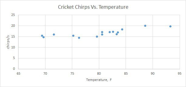
In order to work with some examples we need sample data. There are many data sources available on the internet. For instance, a great source is college Cengage, that have several sets with data pairs meant for linear regression problems. For our example, we are going to use Cricket Chirps Vs. Temperature data where each data point consists of chirps/sec and temperature in degrees Fahrenheit. You can send data in three formats: excel, mtp and ASCII. Let’s download excel data where we can immediately draw graph and see what’s going on.
Right away, in excel, we can additionally do some analysis. For this, we need to click on the excel chart, then go to appeared DESIGN tab and select Add Chart Element and select Trend Line -> Linear.
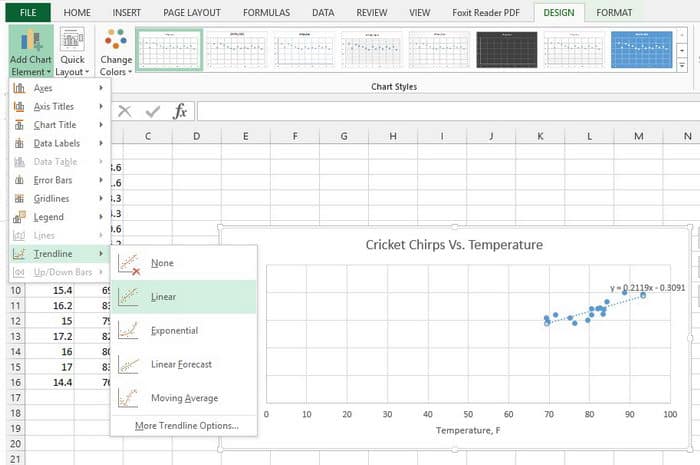
Excel automatically adds trend line, which is nothing more than linear regression. You can select Format Trendline, where you can check Display Equation on the chart check box. As you can see, for our data set linear regression formula is
y = 0.2119x-0.3091
What does this mean practically? We have learned two linear formula coefficients, 0.2119 and 0.3091, that can be used to predict cricket chirp frequency at any given temperature. For instance, we can take any temperature from the range and even out of it and calculate the chirp/sec value. As an example, let’s take temperature 85F according to the formula; we get
y = 0.2119 · 85 – 0.3091 = 17.7Hz.
Another example. We can try to speculate with values out of range. For instance, we would like to know the chirp frequency when the temperature is 50F. Again let’s apply our learned formula and calculate:
y = 0.2119 · 50 – 0.3091 = 10.29Hz
So we have a simple machine which can approximately predict values on given parameter.
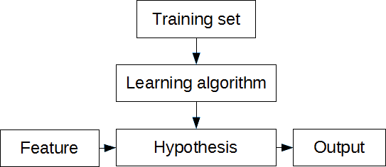
In this example, temperature values we call features and chirp/sec values – target variables or. Continuing with machine learning lexicon, the data set we used for training linear regression parameters is called the training set. The formula we used for trend line is called a hypothesis. The only thing missing here is learning algorithm.
In excel, this process is hidden but is suitable for simple problems like this. And as you already guessed, you can use different types of trend lines (logarithmic, exponential, polynomial, power, etc.) that fit the training set best. Using excel is easy with one variable (univariate) data sets, but when working with multidimensional data, things get more complicated.