Feature extraction from retina vascular images for classification

Classifying medical images is a tedious and complex task. Using machine learning algorithms to assist the process could be a huge help. There are many challenges to make machine learning algorithms work reliably on image data. First of all, you need a rather large image database with ground truth information (expert’s labeled data with diagnosis information). The second problem is preprocessing images, including merging modalities, unifying color maps, normalizing and filtering. This part is important and may impact the last part – feature extraction. This step is crucial because on how well you can extract informative features, depends on how well machine learning algorithms will work.

Dataset

To demonstrate the classification procedure of medical images the ophthalmology STARE (STructured Analysis of the Retina) image database was pulled from https://cecas.clemson.edu/~ahoover/stare/. The database consists of 400 images with 13 diagnostic cases along with preprocessed images.

For classification problem we have chosen only vessels images and only two classes: Normal and Choroidal Neovascularization (CNV). So the number of images was reduced to 99 where 25 were used as test data and 74 as training.

Feature extraction

Vessel images are further binarized – converted to two levels where white color represents vessels and black background. We used Histogram of Oriented Gradient features (HOG) that can be used in a machine learning algorithm. The idea of HOG is to divide the image into smaller blocs wherein each block image gradients are calculated:

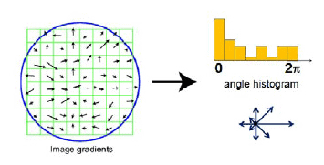
It is essential to decide what size of image blocs are going to be used. If blocks are tiny, you end up with lots of shape information, if blocks are two big – there maybe not enough of shape information. For instance, in our case we have tested three cell sizes: [8 8], [4 4] and [2 2]:

So all features from images were extracted using matlab code:

extractHOGFeatures(img,'CellSize',[4 4]);

Classifying

We have chosen three classification algorithms (Fit k-nearest neighbor classifier, Train binary support vector machine classifier, and binary classification decision tree) to compare performance and select most accurate.

First, we train three classifiers:

classifier1 = fitcknn(trainFeatures, trainLabels);

classifier2 = fitcsvm(trainFeatures, trainLabels);

classifier3 = fitctree(trainFeatures, trainLabels);

Then we try to predict labels with train data:

predictedLabels1 = predict(classifier1, testFeatures);

predictedLabels2 = predict(classifier2, testFeatures);

predictedLabels3 = predict(classifier3, testFeatures);

Results

When we have predictions, we can compare them with real labels of train data. For this we build a confusion matrix for each classifier and calculate precision, recall, Fscore and accuracy metrics:

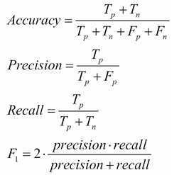
Table 1. Comparison of three classifiers

	kNN			SVM			Dtree
	TP	FN		TP	FN		TP	FN
	5	2		3	4		3	4
	8	10		9	9		11	7
	FP	TN		FP	TN		FP	TN
Precision	0.6349			0.4643			0.4087
Recall	0.609			0.4712			0.4253
Fscore	0.6217			0.4677			0.4169
Accuracy	60%			48%			40%

As we can see kNN based classification algorithm performs best when comparing FScore and accuracy metrics.

Conclusions

This exercise aimed to demonstrate steps of how machine learning algorithm can be implemented for classifying medical images. The task is oversimplified in terms of feature extraction, and classification algorithm application. We have limited features to a single method – Histogram of Oriented Gradient (HOG) which may be limited in finding other attributes.

For grayscale or color images there could also be color distribution used as features. Also other more complex feature extraction methods could be used such as wavelet transformation coefficients.

We have used a tiny image database with only two classes. This, of course, leads to poor classification results. The database size should be comparable to feature vector length to reach decent accuracy. But still, with kNN classifier, we were able to achieve 60% accuracy.

Matlab Algorithm code with the dataset (dataset.zip ~0.7Mb)