


Logistic regression is the next step from linear regression. The most real-life data have a non-linear relationship; thus, applying linear models might be ineffective. Logistic regression is capable of handling non-linear effects in prediction tasks. You can think of many different scenarios where logistic regression could be applied. There can be financial, demographic, health, weather, and other data where the model could be implemented and used to predict subsequent events on future data. For instance, you can classify emails into spam and non-spam, transactions being a fraud or not, and tumors being malignant or benign.
In order to understand logistic regression, let’s cover some basics, do a simple classification on data set with two features, and then test it on real-life data with multiple features.
Sigmoid function kernel
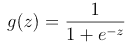
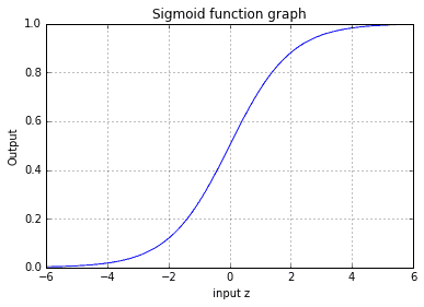
Since logistic regression-based classifier is non-linear, we need a non-linear kernel function. Logistic regression uses a sigmoid function which is “S” shaped curve. It can have values from 0 to 1, which is convenient when deciding to which class assigns the output value.
Using python, we can draw a sigmoid graph:
import numpy as np
import matplotlib.pyplot as plt
z = np.arange(-6, 6, 0.1);
sigmoid = 1/(1+np.exp(-z));
fig = plt.figure('Cost function convergence')
plt.plot(z,sigmoid)
plt.grid(True)
plt.xlabel(' input z')
plt.ylabel('Output')
plt.title('Sigmoid function graph')
plt.show()
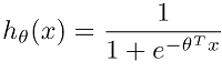
To make a hypothesis out of sigmoid, we need to substitute the z parameter with a vectorized form of ΘTx, representing input features and parameters (weights). Where,
ΘTx = Θ0+Θ1x1+Θ2x2+…+Θnxn
Note: ΘTx can be constructed differently using mapping of features to meet training set structure.
So we can write a hypothesis in compact form:
Logistic regression cost function and gradient descent
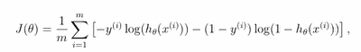
Simply speaking cost function is similar to the linear regression cost function, where the linear hypothesis is replaced with a logistic hypothesis. Without proof cost function can be represented as follows:
To minimize cost function we need to use gradient function:
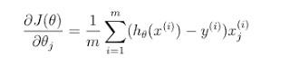
We need to minimize J(Θ) we run a gradient descent algorithm where each Θ is adjusted during several iterations until it converges.
We can write a cost and gradient functions python code:
def cost(theta, X, y):
    '''  logistic regression cost    '''
    sxt = sigmoid(np.dot(X, theta));
    mcost = (-y)*np.log(sxt) - (1-y)*np.log(1-sxt)
    return mcost.mean()
def gradient(theta, X, y):
    '''  logistic regression gradient    '''
    sxt = sigmoid(np.dot(X, theta))
    #label and prediction difference
    err = sxt - y
    grad = np.dot(err, sxt) / y.size # gradient vector
    return grad
To minimize the cost function, we have two ways – write our loop where we step-by-step update theta parameters until getting to the converging point or use built-in optimization routine which takes care of the task. Since we have done manual optimization in linear regression, let’s move on and use tools that make life easier. For optimization, we will use a function called fmin_bfgs which takes cost function, initial thetas, and produce thetas of minimized function. Good news is that we even don’t need to prepare the gradient function.
#create initial theta values
theta = 0.1* np.random.randn(n);
#use fmin_bfgs optimisation function find thetas
theta = opt.fmin_bfgs(cost, theta, args=(XX, Y));
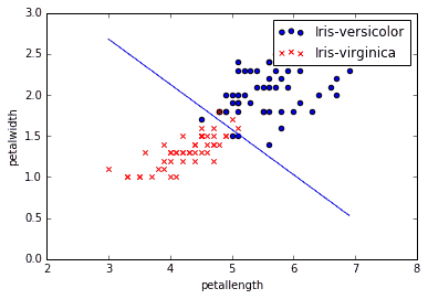
After running minimization we get theta parameters that can be used in classification mode. Visually we can draw a decision boundary on our training data to see where data is separated into classes.
Evaluating logistic regression classifier
We should not take results as granted. We need to test if the model is valid and can be used for classification. We need to set up a test set with known labels. First of all, we can write a predictor function which would produce class 0 if the probability of hypothesis output is h<0.5 and class 1 if the output is h>=0.5.
def predict(theta, X):
    #test new data
    m, n = X.shape
    p = np.zeros(shape=(m, 1));
    h = sigmoid(X.dot(theta.T));
    p = 1*(h>=0.5);
    return p
Then we can prepare some test data to ensure the classifier works OK.
#test classifier with some random data
XXX = np.array([[1.0, 5.0, 1.4], #0
                [1.0, 1.4, 2.0], #0
                [1.0, 7.0, 1.0]]); #1
print(predict(theta, XXX));
And finally, we can run our code on training data or separate validation sets to see classification accuracy.
#test on labeled data
p = predict(theta, XX);
print ('Accuracy: %f' % ((Y[np.where(p == Y)].size / float(Y.size)) * 100.0));
As we can see, accuracy is 94%.
We can double-check the model on data by using WEKA software by selecting the same data and Logistic classifier:
We can see that using the same model in WEKA also gets 94% accuracy.
Next time we will touch the more complicated case of Logistic regression which includes regularization and multidimensional sets. As you dig deeper, you will find that logistic regression is only one of many available classification tools.
If you want to test the algorithm by yourself, here is logistic_regression.zip of python code and dataset, or use python assignment help.